CNN Components for Medical Imaging: What Kernels, Pooling, and Receptive Fields Actually Do

A primer on the four CNN primitives — kernels, conv layers, pooling, receptive fields — grounded in real activations and Grad-CAMs from a chest X-ray classifier.

June 1, 2026Saianiruth M

A convolutional neural network is a stack of learned local filters. Each filter scans its input for a specific pattern and outputs a map of where that pattern appeared. Layers stack so deeper filters compose patterns from earlier ones, and spatial resolution is reduced between stages so a neuron near the top of the network sees a much larger region of the input than one near the bottom.

The rest of this post is what each piece — kernels, conv layers, pooling, receptive fields — actually does on a chest X-ray, and what happens when one of them doesn't fit your problem.

Why convolutions exist

A 224×224 grayscale image has roughly 50,000 pixels. Send it through one fully-connected layer with 1,024 hidden units and you've burned 50 million weights — absurd, and the wrong inductive bias besides. Useful pixel correlations in images are mostly local: a rib edge is defined by a few neighboring pixels, not by the top-left corner and the bottom-right.

Convolutions encode three priors that match images well:

Locality. Each output depends only on a small neighborhood of the input.
Weight sharing. The same filter applies everywhere. A consolidation in the right upper lobe and one in the left lower lobe activate the same feature detector — the network doesn't relearn "consolidation" separately for every pixel position.
Translation equivariance. Shift the input and the feature map shifts the same way.

Throughout this post we'll come back to one pediatric chest radiograph from the Kermany et al. (2018) pneumonia dataset:

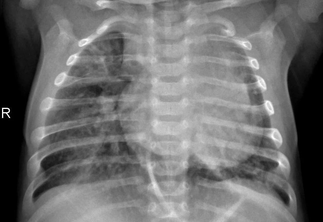
Pediatric chest X-ray with visible lower-zone opacity, used as the canonical input throughout this post. — The pediatric AP chest X-ray used throughout. Lower-zone opacity consistent with pneumonia. Every activation, receptive field, and Grad-CAM below is computed on this exact image. The dataset is pediatric, so the model is not a general adult-CXR classifier — but the concepts apply.

The model is a ResNet50 pretrained on ImageNet with the final layer swapped for a 2-class head and fine-tuned for 10 epochs. Test accuracy 89.7% — a teaching example, not a clinical one.

The mechanics

Kernels

A 3×3 kernel is nine numbers. The convolution operation slides it across the image, multiplying each kernel value by the corresponding input pixel and summing, producing one output value per position. With padding, the output is the same size as the input.

The clearest way to see what convolution computes is with a hand-designed kernel. Here is a Sobel-x kernel — positive values on the right, negative on the left — applied to a chest radiograph:

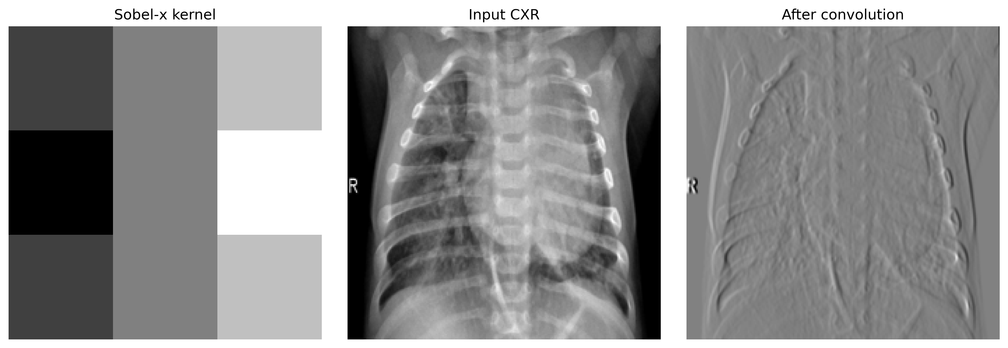
A 3x3 Sobel-x kernel (left) applied to a pediatric chest X-ray (center), producing an output (right) with strong response on vertical edges including ribs, mediastinum, and the side marker. — A 3×3 Sobel-x kernel applied to a CXR. The output is strong wherever the input transitions horizontally from dark to bright — ribs, the mediastinum, and notably the "R" side marker. CNN kernels do exactly this; the difference is that the nine numbers are learned via gradient descent, not designed.

Notice the marker. The Sobel kernel doesn't care that "R" is an annotation rather than anatomy — it responds to whatever edges exist. Learned kernels inherit the same property, and we'll come back to it.

Early-layer learned kernels typically look like edge, color, and gradient detectors. Deeper layers compose these into textures, parts, and eventually full anatomical structures.

Conv layers

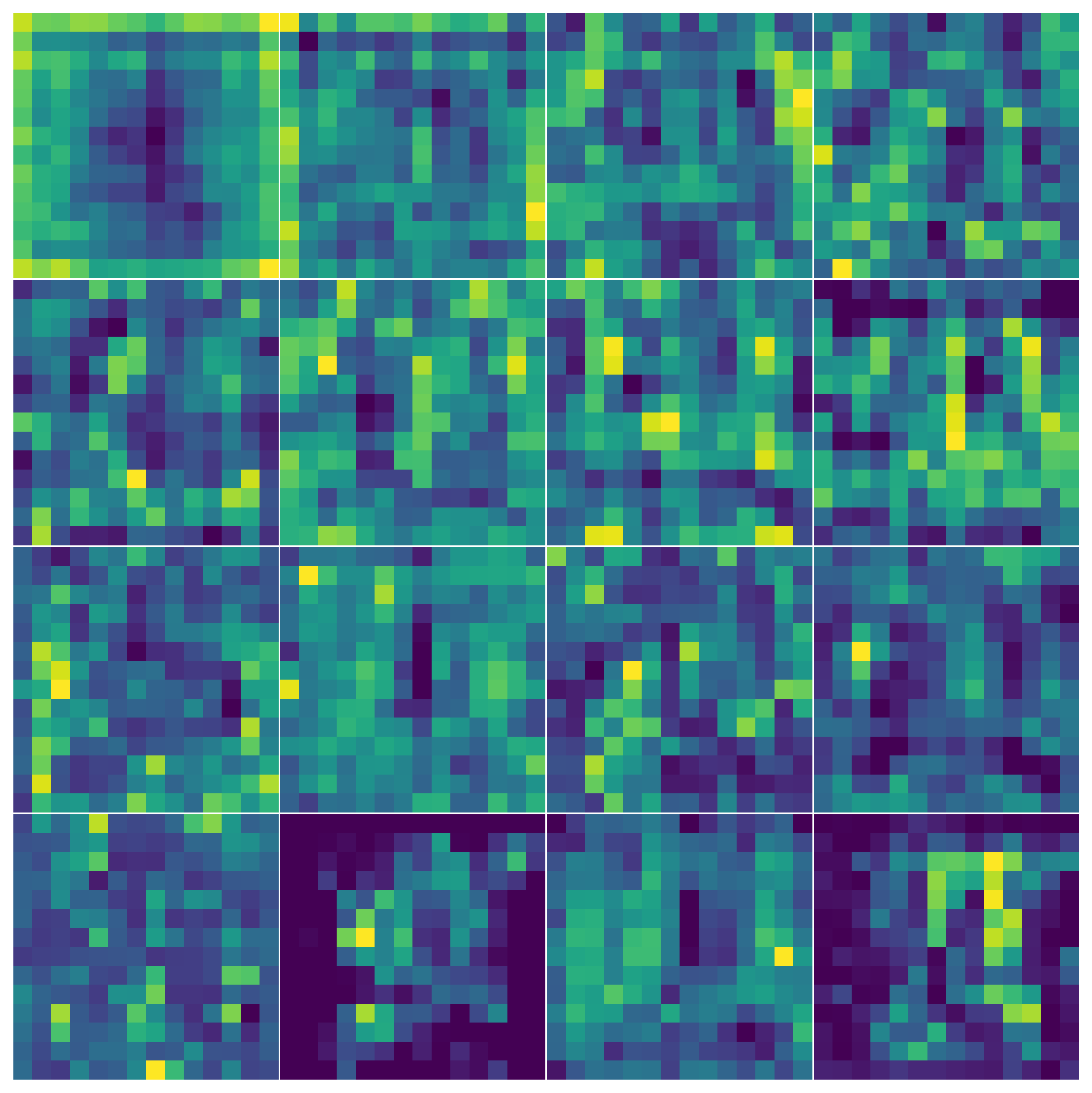
A conv layer applies many kernels in parallel, each producing one output channel. ResNet50's first conv layer has 64 kernels of size 7×7. Here is what they look like after ImageNet pretraining:

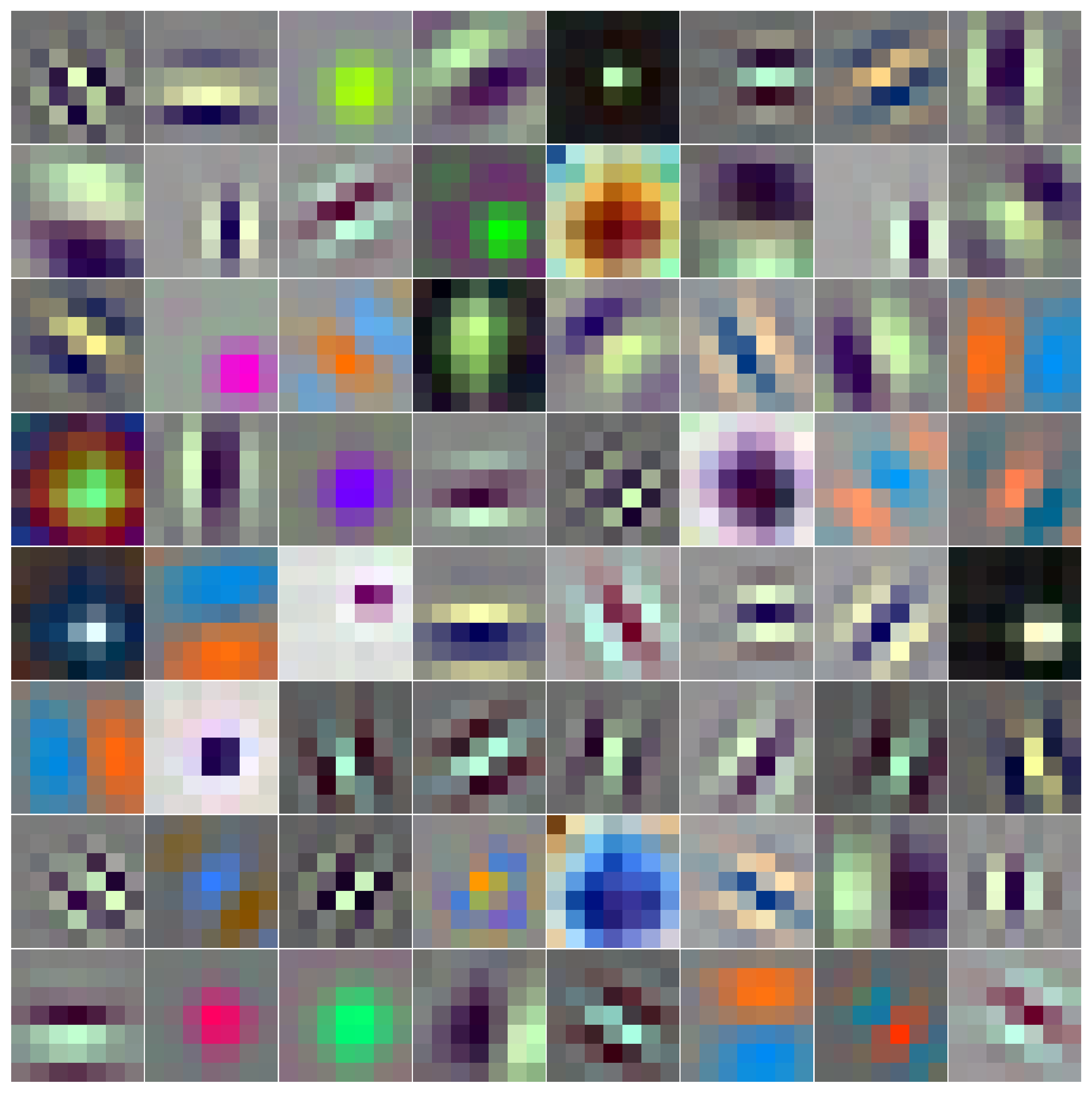
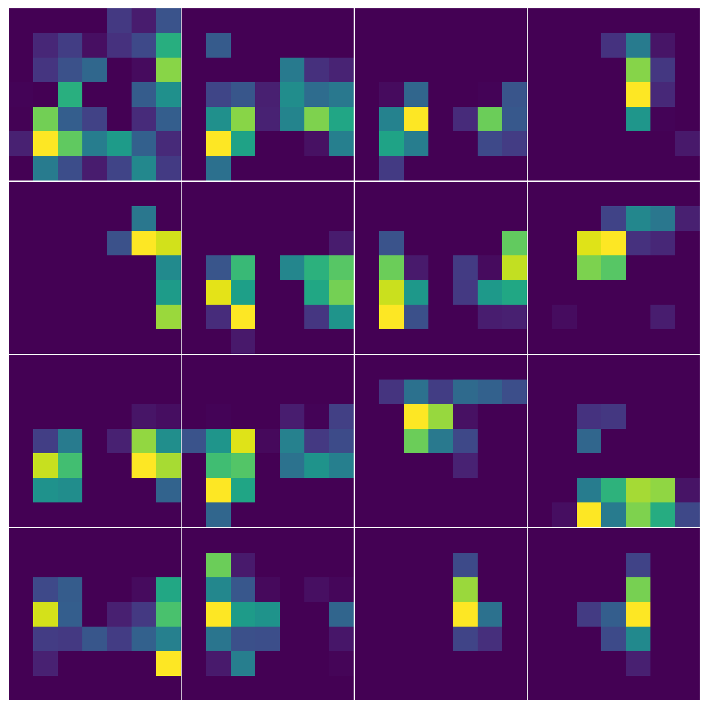
A grid of 64 first-layer 7x7 kernels from ResNet50 pretrained on ImageNet, showing oriented edge detectors and color-gradient patterns. — First-layer kernels in ResNet50 pretrained on ImageNet. Mostly oriented edge detectors and color/gradient patterns.

And here are the same kernels after fine-tuning for 10 epochs on the pneumonia dataset:

The same grid of first-layer ResNet50 kernels after fine-tuning on chest X-ray data, visually nearly identical to the ImageNet-pretrained version. — The same first layer after 10 epochs of CXR fine-tuning. The relative L2 change in weights was 0.5%.

They look identical because they essentially are. Early-layer features — edges, blobs, gradients — are general. They don't need to change much when you transfer between domains. The work of adapting to medical imaging happens deeper in the network. This is also why almost every production CXR system initializes from ImageNet weights rather than training from scratch.

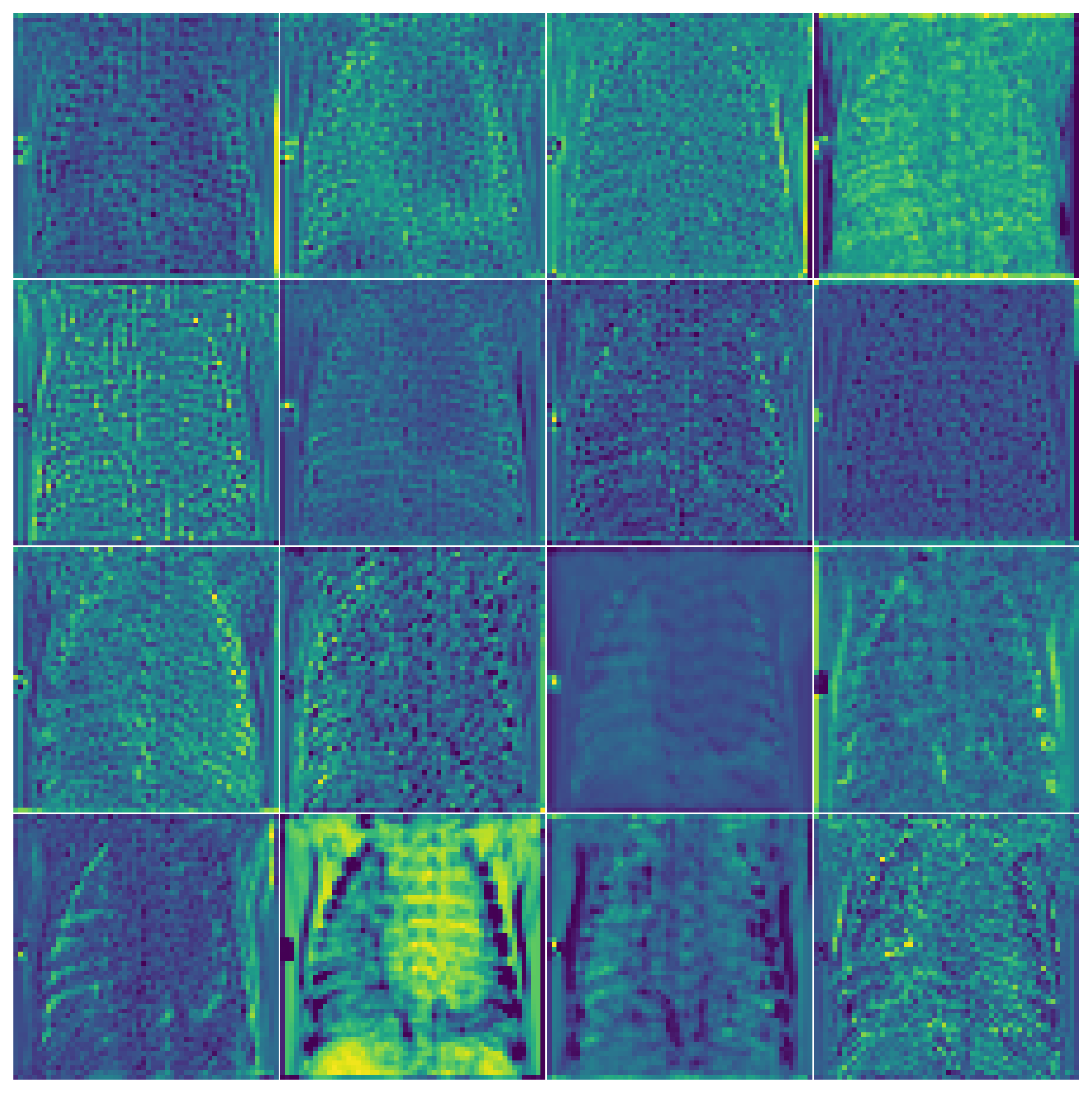
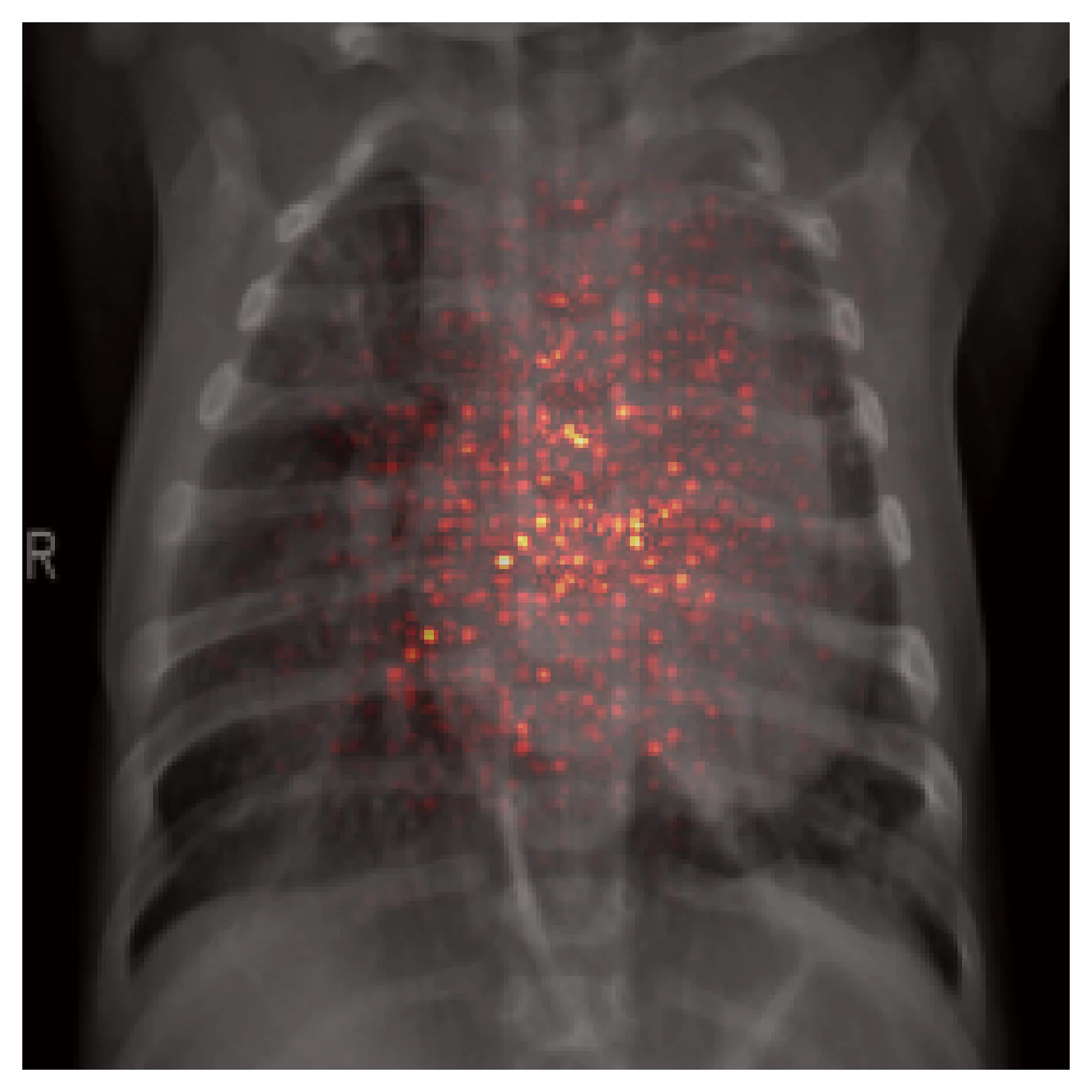
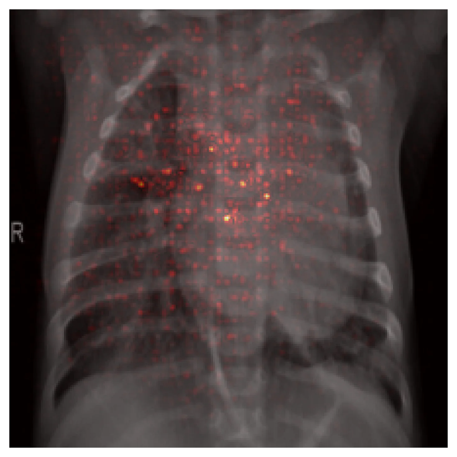
You can watch abstraction grow with depth by reading off activations at three layers of the same model on the same input:

A grid of 16 channel activation maps from ResNet50 layer1, with spatial detail still visible — ribs, chest cavity, the side marker. — Top-16 active channels at layer1 (56×56). You can still see the chest cavity, the ribs, and the marker. Features are local and spatial.

A grid of 16 channel activations at ResNet50 layer3, showing 14x14 maps with blocky semi-localized firing patterns. — Layer3 (14×14). Spatial resolution has collapsed. Channels are firing on what look like mid-level part features.

A grid of 16 channel activations at ResNet50 layer4, with very sparse 7x7 maps where each channel responds to only a few specific cells. — Layer4 (7×7). Extremely sparse. Each channel responds to a few specific concepts. This is what the classification head reads.

Pooling

Pooling reduces the spatial size of a feature map. We do it for three reasons: to reduce compute, to give the network a small amount of translation invariance, and to force later layers to summarize rather than enumerate.

Max-pool takes the maximum activation in each window. Avg-pool takes the average. They preserve different things:

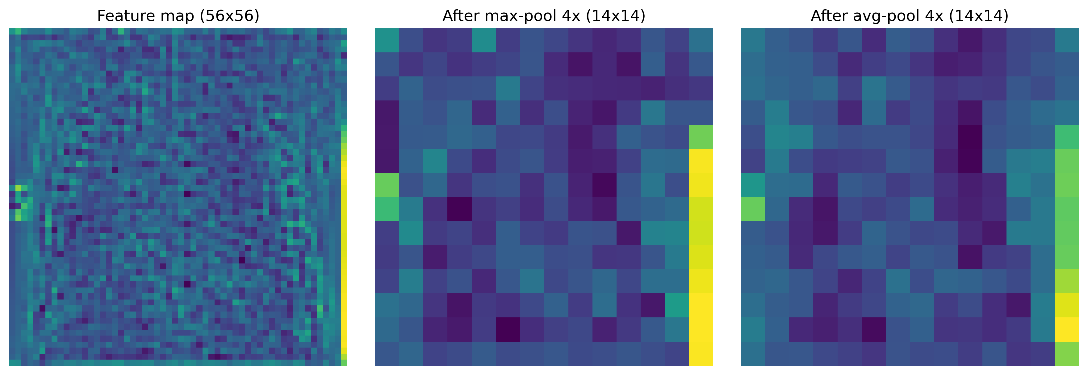
One feature map at 56x56 shown before pooling, after 4x max-pooling at 14x14, and after 4x average-pooling at 14x14. — Same feature map, before pooling (left), after 4× max-pool (center), and after 4× avg-pool (right). Max preserves peaks. Avg smooths and dampens.

Max is the default in classification CNNs because pathology signals are often peaky — a bright opacity against dark lung field, a thin fracture line against bone — and avg can wash those out. The cost: anything subtler than the pool window vanishes. A 2-pixel-wide line in a 4×4 max-pool window survives if it is a strong edge and disappears if it is faint.

Receptive fields

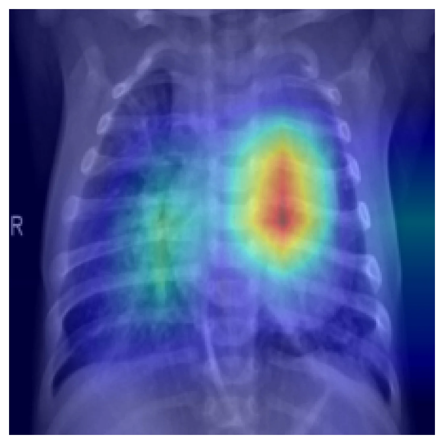
The theoretical receptive field of a neuron is the region of the input image that can influence its value. At layer4 of ResNet50, this is essentially the entire image. But the effective receptive field — where the input actually has weight, measured as gradient magnitude with respect to input pixels — is much smaller and roughly Gaussian (Luo et al., 2016).

Here is the effective RF for a neuron at the center of three different layers, computed on the same input:

Effective receptive field at layer1 of ResNet50, shown as a small concentrated dot near the center of the chest radiograph. — Effective RF at layer1. A small concentrated dot — the neuron sees only its immediate neighborhood.

Effective receptive field at layer3, scattered across the central chest cavity but still concentrated. — Layer3. Scattered across the central chest cavity, but still concentrated.

Effective receptive field at layer4, spread broadly across most of the chest area. — Layer4. Spread across the chest, but still not uniform.

The practical consequence: if you are trying to detect findings smaller than the effective RF resolution at the layer you read features from, the signal is diluted by pooling before the classifier sees it. The standard fix is a feature pyramid (FPN, BiFPN) or a U-Net-style decoder, where you read from earlier, higher-resolution layers in parallel with the deeper ones.

Where it shines, where it breaks

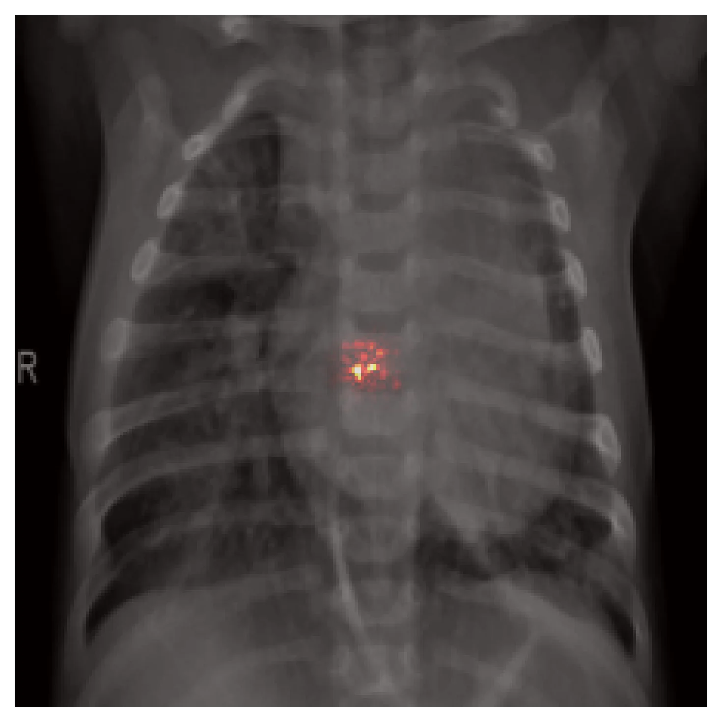
CNNs are excellent at locally-defined, texture-rich pathologies — consolidation, effusion, infiltrate. The inductive biases match the data. Here is Grad-CAM on the same input as above, with the model correctly classifying it as pneumonia:

Grad-CAM heatmap overlaid on a chest X-ray, with strong activation localized over consolidated lung tissue on one side of the chest. — Grad-CAM at layer4 for the pneumonia class. The model has localized on the side of the chest where there is visible opacity. Correct prediction, clinically reasonable explanation.

CNNs break in three predictable places.

Small findings. A hairline fracture, a small nodule, or a thin pneumothorax line can be a handful of pixels in the input. After several pooling stages, the signal is gone before the classifier sees it. The fixes are architectural — FPN, BiFPN, higher input resolution, segmentation heads on early layers — not hyperparameter tweaks.

Long-range reasoning. Cardiomegaly is defined by comparing heart silhouette to thoracic cavity width. Mediastinal shift requires comparing left and right hemithoraces. CNNs can do this only by stacking enough layers to span the spatial range; transformers can do it in one attention step. This is part of why ViTs and hybrid CNN-transformer models started showing up in medical imaging.

Shortcut learning. Trained on data with spurious correlations, a CNN will happily learn the shortcut instead of the pathology. Here is an example from the same model on a different correctly-classified pneumonia case:

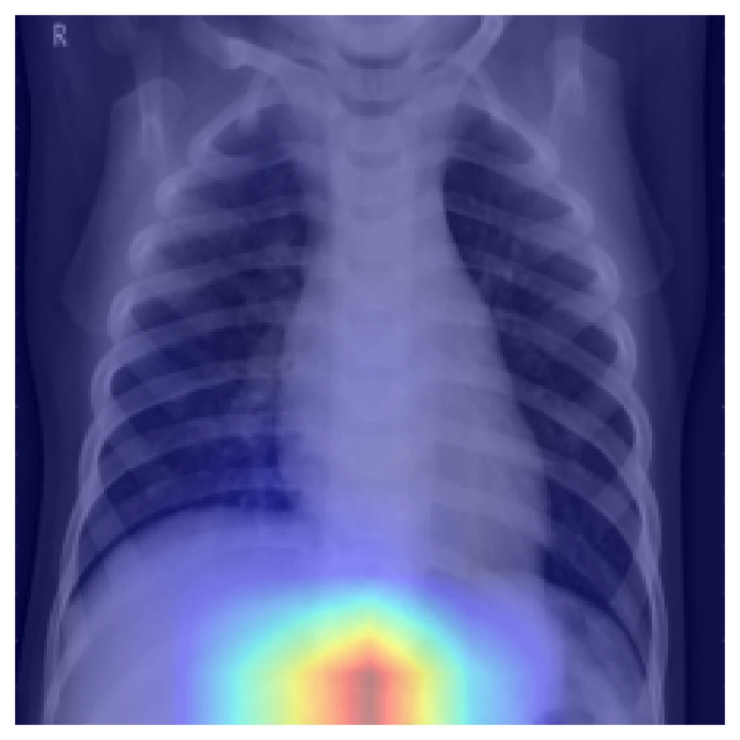
Grad-CAM overlay on a chest X-ray where the heatmap is concentrated below the lung field, on the upper abdomen and diaphragm region. — A different correctly predicted pneumonia case. The model's attention is concentrated below the lungs, on the upper abdomen and diaphragm — not on lung tissue. Correct prediction, wrong explanation.

The prediction is right; the reasoning is wrong. Markers, tubes, exposure differences, side-letter tokens, even patient positioning can become shortcuts if they correlate with the label across the training set. A held-out split from the same distribution will not catch this — only attribution methods will, and only if you actually run them.

How this shows up in production medical-imaging engineering

Backbone selection rarely comes down to top-1 ImageNet accuracy. The relevant questions are whether the effective RF covers the finding size at the depth where the head reads features, how much input resolution you can afford, and which features need to be available at which scale.

Debugging matters at least as much as benchmarking. Two CNNs with identical test AUC can have wildly different attribution patterns. Grad-CAM is cheap; running it on a sample of test cases — especially errors — surfaces shortcut features that accuracy curves hide.

Small findings are an architecture problem, not a tuning problem. If pathology is smaller than the effective RF resolution at the layer you read from, no learning-rate schedule fixes that. Reach for feature pyramids, higher input resolution, or a detection-oriented architecture before tuning hyperparameters.

External validation is the honest measurement. Accuracy on a held-out split from the training distribution is a weaker signal than most teams treat it as. The first time a CXR model meets data from a different scanner, hospital, or patient population is usually the first time its real-world reliability is honestly measured.