BCE vs Focal Loss for Medical Imaging: Three Losses on a 58:1 Imbalance
Binary cross-entropy, weighted BCE, and focal loss compared on synthetically-imbalanced CXR classification. What the curves promise versus what the test set delivers.
Binary cross-entropy measures the negative log-likelihood that a model assigned to the true class for each example. Focal loss multiplies that by a (1 − p_t)^γ factor that down-weights examples the model already gets right. Weighted BCE multiplies it by a per-example weight that up-weights the minority class. All three are pointwise modifications of the same idea; the differences show up under class imbalance.
Why class imbalance matters
In medical imaging, positives are rare. A chest X-ray screening cohort might be 99% normal. A multi-disease classifier sees five orders of magnitude fewer cardiomegaly cases than no-finding cases. An object detector trained on RSNA pneumonia sees thousands of negative anchor positions per positive box.
The problem is the loss surface. Vanilla BCE sums one per-example loss across the batch. If 99 out of 100 examples are negative and the model has learned to predict "negative" with reasonable confidence, the 99 easy examples each contribute a small but nonzero loss. Together they swamp the gradient signal from the one positive example. Training stalls on a "predict the majority" solution that scores well on accuracy but is clinically useless.
Three remedies exist. Up-weight the minority class so its losses count more (weighted BCE). Down-weight examples the model is already confident about, regardless of class (focal loss). Or change the data — oversample the minority, undersample the majority. This primer focuses on the loss-side fixes.
The mechanics
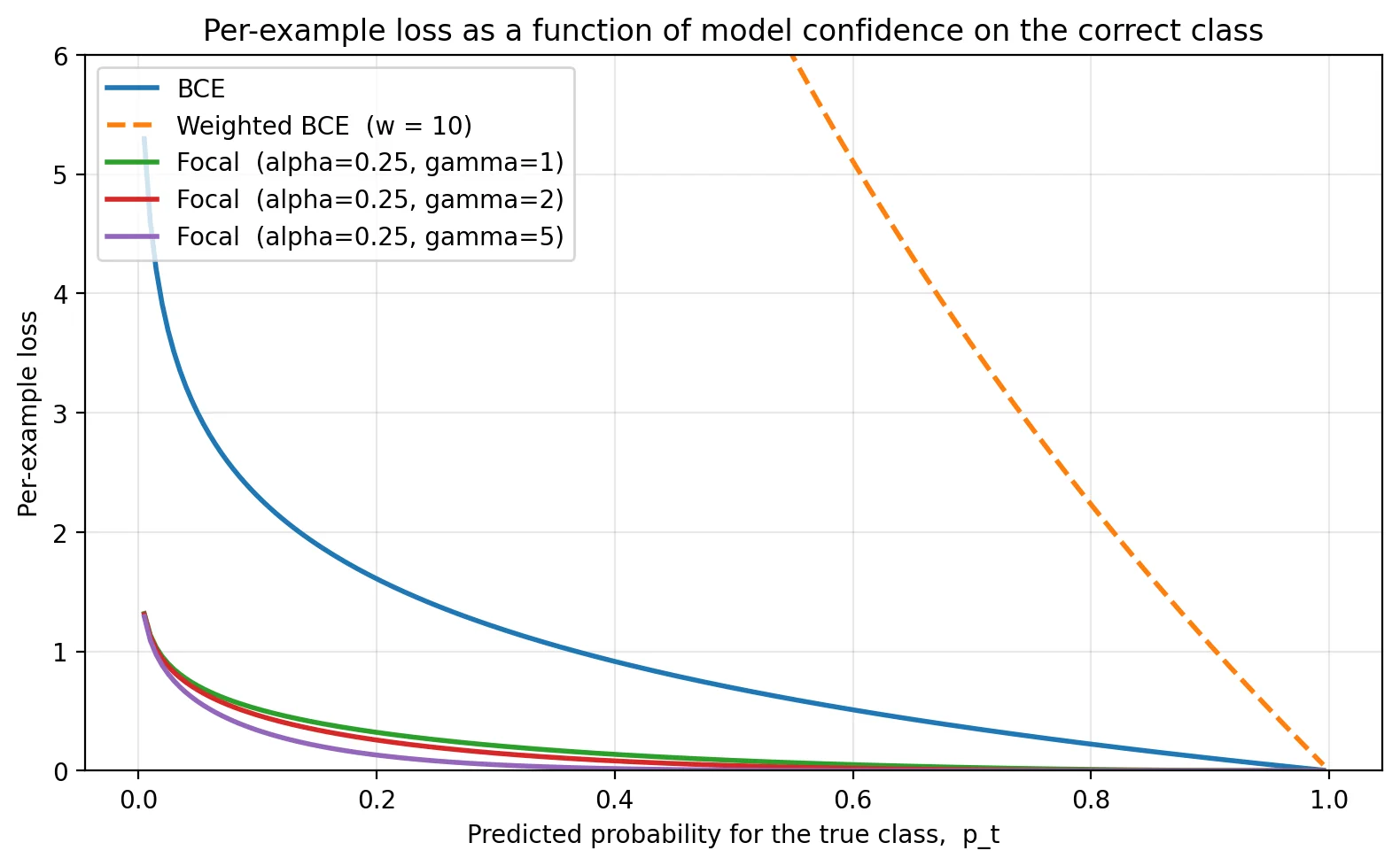
Define p_t as the probability the model assigned to the true class for an example: p_t = p if y = 1, else 1 − p. The three losses are:
BCE:    L = -log(p_t)
WBCE:   L = -w_y · log(p_t)             # w_y depends on the class
Focal:  L = -α · (1 - p_t)^γ · log(p_t) # α, γ are scalars
For BCE, the loss depends only on how confident the model was on the correct class. For weighted BCE, that same loss is scaled by a per-class constant. Focal loss multiplies BCE by (1 - p_t)^γ, which is near 0 when the model is confident (p_t ≈ 1) and near 1 when it's not (p_t ≈ 0). The α scalar in focal is a class-balancing weight similar in spirit to weighted BCE's w_y.
What this looks like on the real line:
The story is even clearer in the gradient:
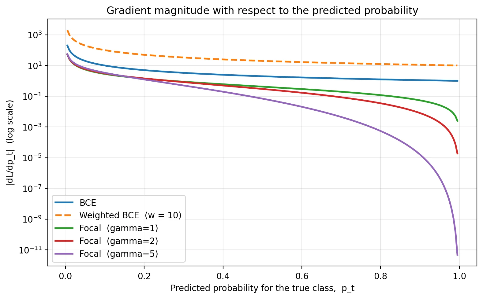
|dL/dp_t|, log y-axis. At p_t = 0.99, BCE still produces a gradient of ≈ 1. Focal with γ=2 produces ≈ 1e-5. The whole point of focal loss is making confident-correct examples invisible to backprop.The three losses in PyTorch:
import torch
import torch.nn.functional as F
from torchvision.ops import sigmoid_focal_loss

# BCE
loss = F.binary_cross_entropy_with_logits(logits, targets)

# Per-sample weighted BCE: up-weight the minority class
w = torch.where(targets == 0, minority_weight, 1.0)
loss = F.binary_cross_entropy_with_logits(logits, targets, weight=w)

# Focal loss (α = 0.25, γ = 2 are the values from the RetinaNet paper)
loss = sigmoid_focal_loss(logits, targets, alpha=0.25, gamma=2.0, reduction="mean")
What actually happens
The theory above predicts focal should dominate at high imbalance. Time to check. Take the Kermany pneumonia dataset, subsample NORMAL to 5% of its original count to induce a 58:1 imbalance, train three ResNet50 classifiers from the same ImageNet init for 5 epochs each — one per loss function. Same data, same hyperparameters, same random seed; only the loss differs.
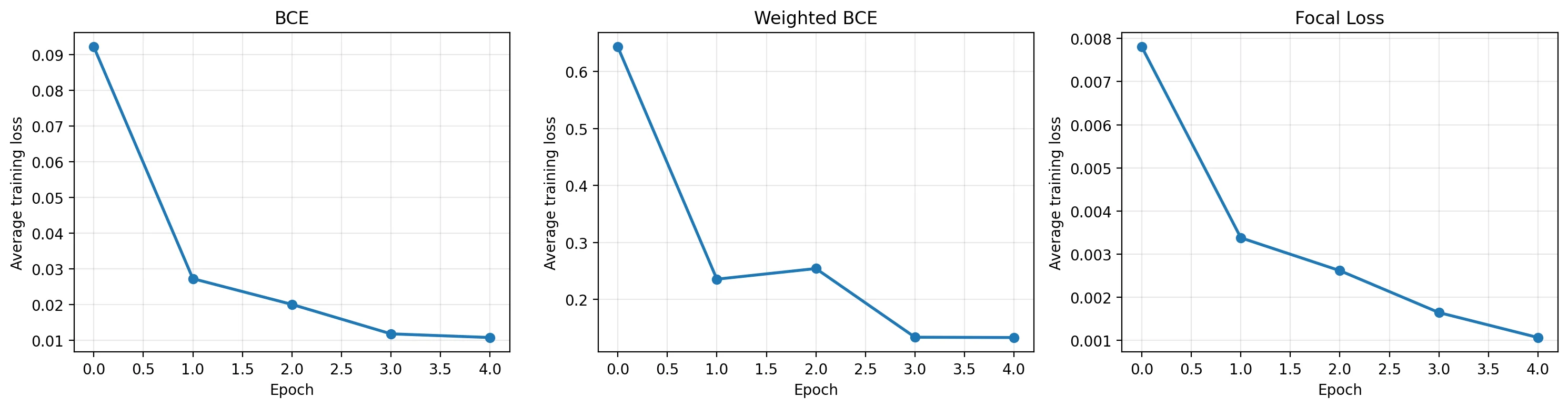
(1 - p_t)^γ factor — so don't compare values across panels. The shapes show all three converge cleanly.The interesting question is what each model does on the test set:
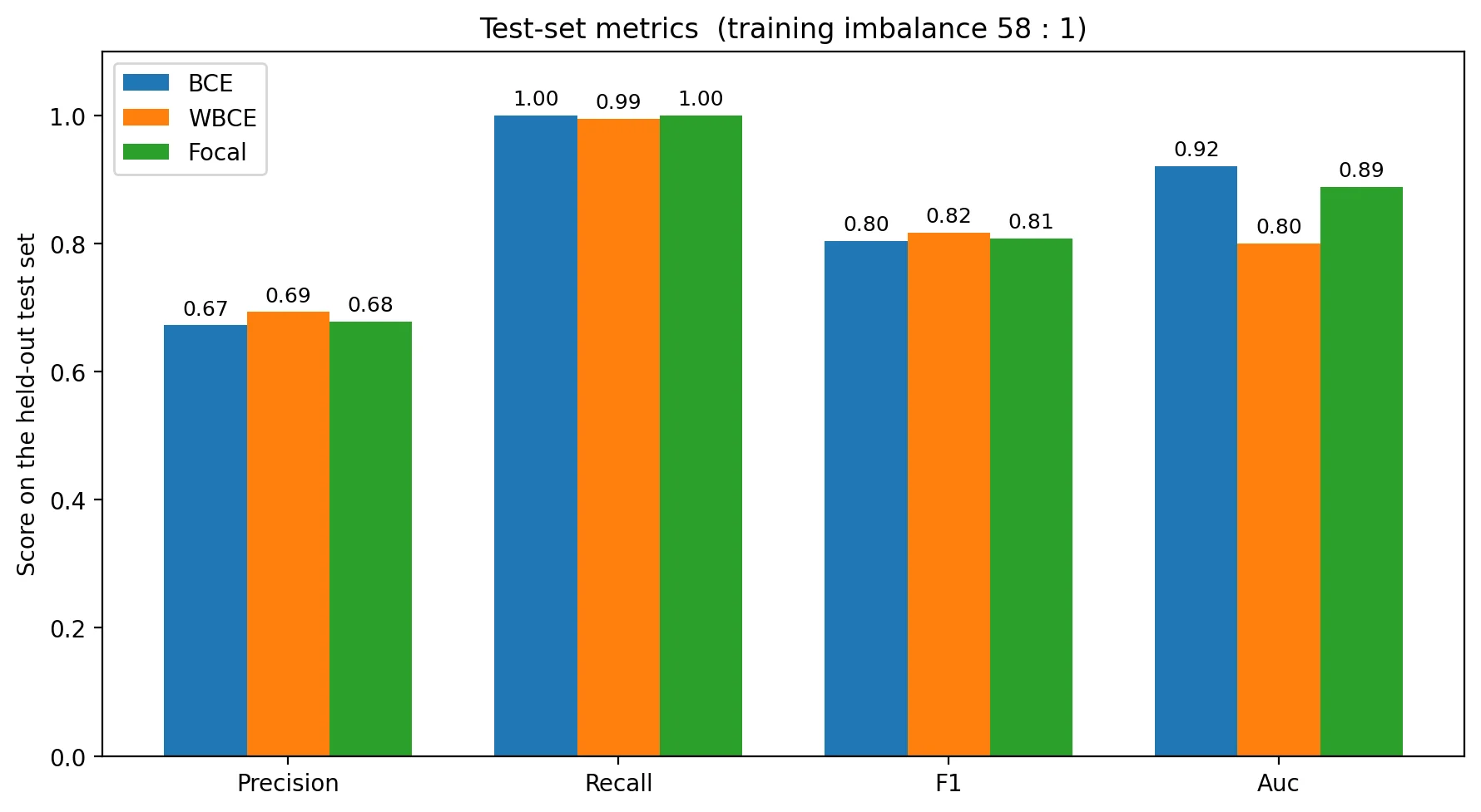
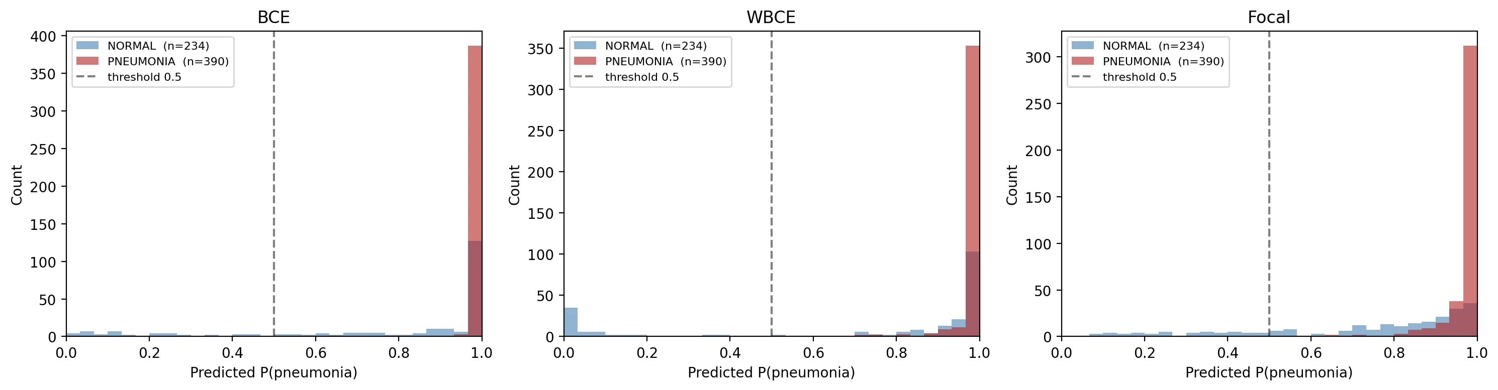
The textbook prediction was that focal would dominate at this imbalance. It didn't. Plain BCE has the highest AUC. Weighted BCE has the best F1 at threshold 0.5 but pays for it in ranking quality.
The confidence distribution explains why:
Two practical observations.
AUC and F1 measure different things. A model can rank correctly (high AUC) while having a badly-calibrated decision threshold (low F1 at 0.5). BCE got the ranking right; weighted BCE got the threshold-0.5 decision right; focal got neither perfectly but was reasonable on both.
Focal loss was designed for a different problem. Lin et al. (2017) introduced focal loss for RetinaNet, a dense detector. At inference time, RetinaNet produces ~100,000 anchor predictions per image, the overwhelming majority of which are easy negatives. Focal was built to make that ocean of easy negatives invisible to the gradient. In classification, there is one prediction per image. The 58:1 imbalance here is significant, but it's not the "thousands of easy negatives per positive" regime that focal addresses. The pretrained ImageNet backbone is also doing most of the discrimination work for us — BCE alone reaches AUC 0.92 because the features are already good.
How this shows up in production medical-imaging engineering
Reach for weighted BCE when the imbalance is moderate (single digits to roughly 100:1) and the task is classification. It's the simplest fix and usually moves precision and recall in the right direction.
Reach for focal loss when the imbalance is structural — dense detection, segmentation with rare classes, multi-label with thousands of negatives per positive. This is what it was designed for, and the gains are real there. In classification with a strong pretrained backbone, the gains often disappear.
Don't trust the loss function to fix calibration on its own. AUC tells you the model can rank; the confidence histogram tells you what the threshold-0.5 cut is actually doing. If you care about precision/recall at deployment, tune the threshold after training rather than relying on the loss to land it.
Look at the confidence distribution before you ship. The bar chart of precision/recall/F1/AUC compresses three rich histograms into four scalars; the histograms surface failure modes that the scalars hide.
Further reading
- Lin, T.-Y. et al. Focal Loss for Dense Object Detection. ICCV 2017. The RetinaNet paper. Section 3 walks through the focal loss derivation; Figure 1 is what the analytical curves above are reproducing.
- Cui, Y. et al. Class-Balanced Loss Based on Effective Number of Samples. CVPR 2019. A more principled approach to per-class weighting than the inverse-frequency heuristic.
- Johnson, J. M. and Khoshgoftaar, T. M. Survey on deep learning with class imbalance. Journal of Big Data, 2019. Broad survey of imbalance-handling techniques across deep learning.
Part of an ongoing series on production medical imaging. The backprop primer covers the gradient mechanics this post builds on; B26's PaliGemma fine-tuning post discusses the same Focal-vs-WCE choice at the 3B classification head. If a loss-function decision is on your roadmap, reach out.