Backpropagation for Medical Imaging: How Gradients Flow Through a CXR Classifier

Backpropagation is the algorithm that computes the gradient of a loss with respect to every parameter in a neural network. It does this by applying the chain rule layer-by-layer, propagating gradients backward from the loss through the computational graph to each parameter. One forward pass to compute predictions and the loss, one backward pass to compute every parameter's gradient — linear in the depth of the network, not exponential.

Why we need it

A modern medical imaging model has tens of millions of parameters. A ResNet50 classifier has about 25 million. To train any of them with gradient descent we need a partial derivative of the loss with respect to each one, on every batch. Without backprop, that would mean either symbolic differentiation (intractable for the size of the computational graph), numerical differentiation (one forward pass per parameter — impossibly expensive), or hand-derived gradient formulas for every architecture (error-prone and architecture-locked).

Backprop gives us all gradients for the price of approximately one forward pass. It has existed since the 1970s, was applied to neural networks by Rumelhart, Hinton, and Williams in 1986, and only became practical at scale in the 2010s when GPUs, large labeled datasets, and a series of architectural and optimization tricks (good initialization, batch normalization, residual connections, Adam) made it possible to actually train networks deep enough to learn rich visual features.

For medical imaging, "deep enough" usually means a pretrained ImageNet backbone with a task-specific head. The backbone provides features; backprop adapts them. The depth of adaptation, as we'll see, is uneven.

The mechanics

The forward pass starts at the input, applies each layer's transformation in sequence, and ends with a loss value. The backward pass starts at the loss, applies the chain rule in reverse to compute the gradient at each layer's output, and uses those to compute the gradient with respect to each layer's parameters. Concretely, if z_i = f_i(z_{i-1}; θ_i) is the output of layer i, then

∂L/∂z_{i-1} = ∂L/∂z_i · ∂z_i/∂z_{i-1}
∂L/∂θ_i    = ∂L/∂z_i · ∂z_i/∂θ_i

PyTorch's autograd builds the computational graph during the forward pass and walks it backward when you call .backward(). The whole training step is unceremonious:

import torch.nn as nn

model = MyNet()
opt = torch.optim.Adam(model.parameters(), lr=1e-4)
loss_fn = nn.CrossEntropyLoss()

for x, y in train_loader:
    # Forward pass: build the computational graph
    pred = model(x)
    loss = loss_fn(pred, y)

    # Backward pass: walk the graph backwards, populate p.grad for every parameter
    opt.zero_grad()
    loss.backward()

    # Apply the gradients
    opt.step()

What backprop actually produces is one number per parameter, every batch. To get a sense of those numbers in practice, here is the per-stage gradient L2 norm on the first batch of pneumonia data, for two ResNet50 variants — one with fresh random initialization, one with ImageNet pretrained weights:

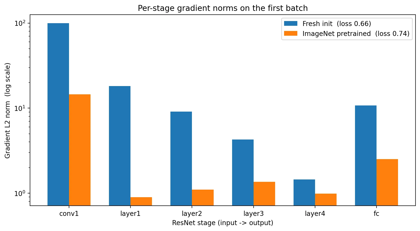
Two observations worth flagging. The textbook story is that gradients vanish with depth in a fresh-init deep network. In ResNet that story is muted: skip connections deliver gradients to early layers efficiently, and conv1 ends up with the largest gradient norm of any stage in both runs. What you do see is the magnitude difference between fresh and pretrained — pretrained weights start near a useful solution, so smaller corrections are needed. The factor of ten difference in gradient norm is why pretrained models converge fast and fresh-init deep networks are difficult to train without all the modern tricks layered together.

Training dynamics in practice

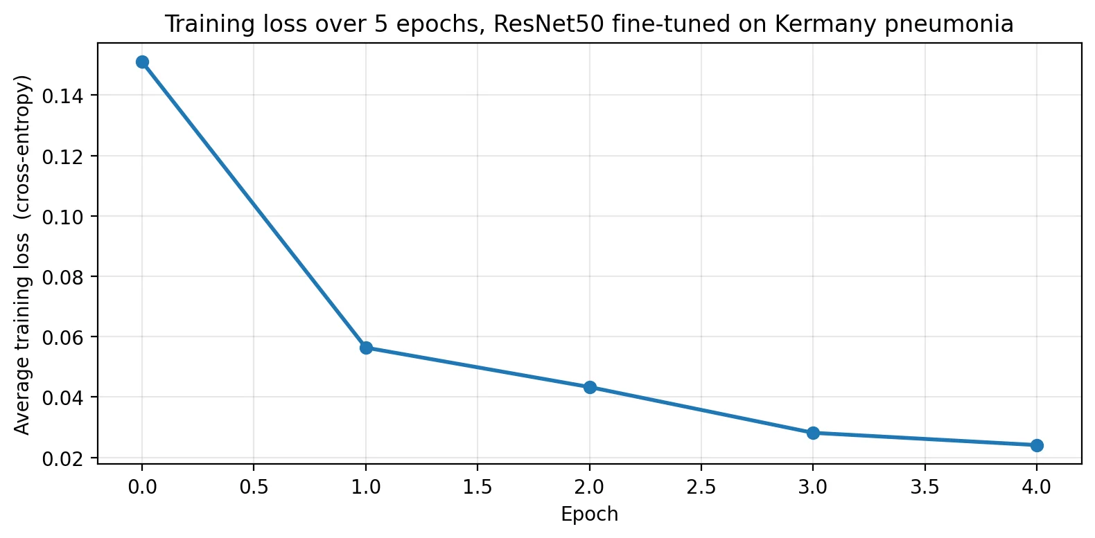
What backprop looks like across an actual training run. Five epochs of fine-tuning the pretrained ResNet50 on Kermany pneumonia data with Adam at lr=1e-4:

The gradient norms themselves shrink as the loss does. Recording the per-stage gradient at the last step of each epoch:

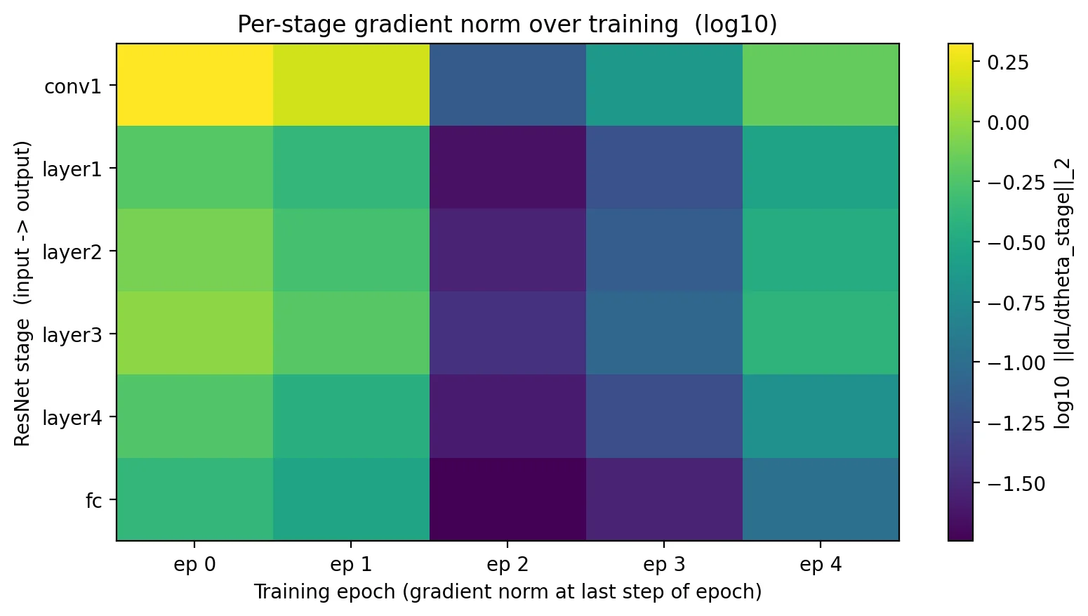
The noise in single-step measurements is a real characteristic of gradient-norm logging. In production training pipelines, the gradient norm logged at each step bounces around the trend by an order of magnitude or more. Smooth before drawing conclusions.

What backprop produced over the full run is a different question: how much did each stage actually change? Cumulative weight change, measured as ||W_final - W_init|| / ||W_init|| per stage:

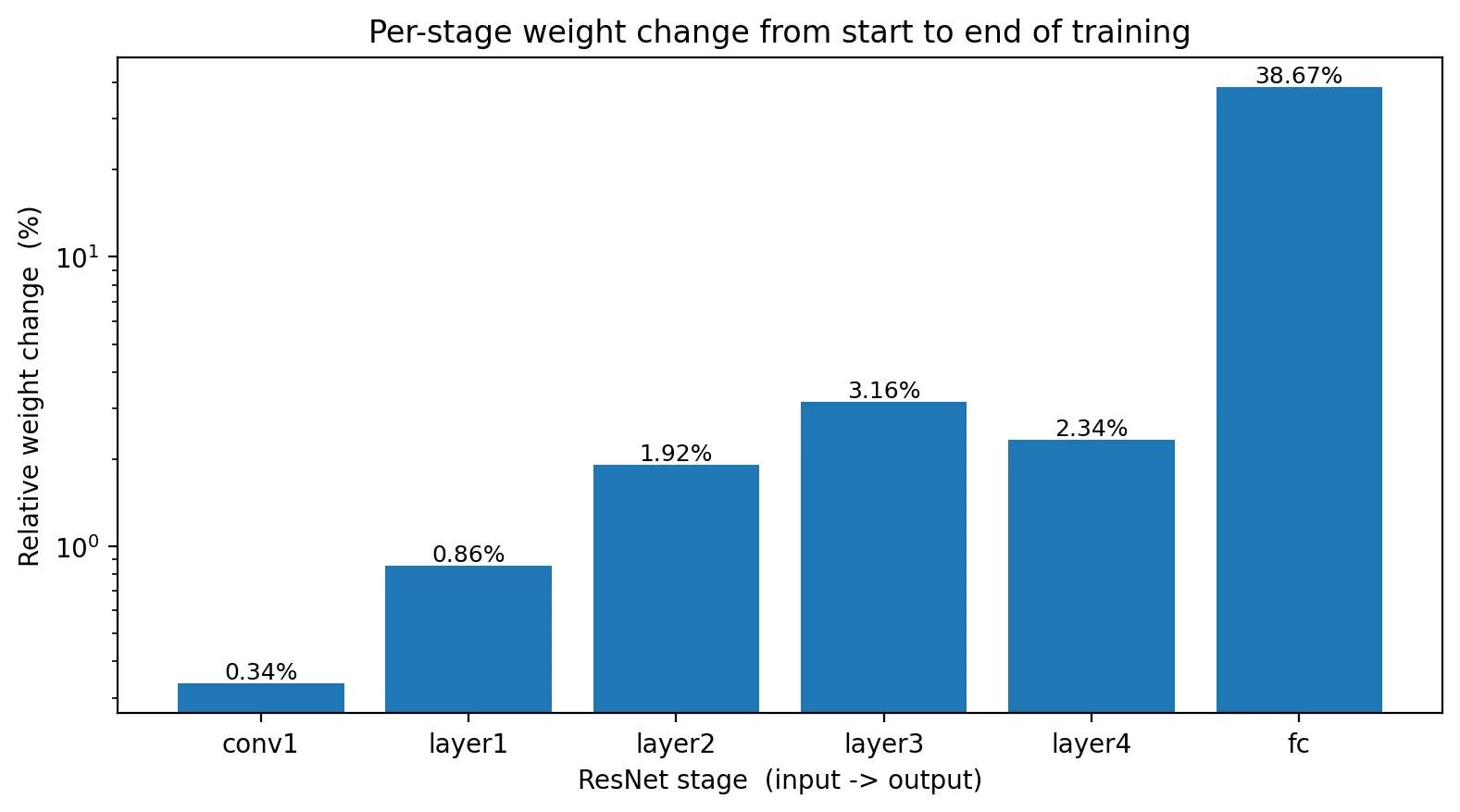
This is the central practical observation: backprop produces gradients at every layer, but the resulting weight changes are highly non-uniform. Early-layer pretrained features are nearly correct already; deeper layers adapt more; the head, which was randomly initialized, changes dramatically. This is the depth-of-adaptation pattern that justifies the standard medical-imaging training recipe: pretrain on natural images, fine-tune end-to-end at a small learning rate, expect the early stages to barely move.

Where it shines, where it breaks

Backprop is universal. Any differentiable model — CNN, Transformer, diffusion model, neural ODE — trains the same way. PyTorch's autograd handles the bookkeeping automatically.

It breaks in a few places worth knowing.

Vanishing or exploding gradients in deep non-residual networks. Pre-ResNet, deep stacks of conv layers had a hard ceiling around 20 layers because gradients either vanished or blew up by the time they reached the input. ResNet's skip connections, batch normalization, careful initialization (Kaiming, Xavier), and gradient clipping are all interventions to keep gradient magnitudes well-behaved as they propagate.

Memory cost. Backprop requires storing all the forward-pass activations to compute the backward pass. For large models or large batches, this is the dominant memory cost — often larger than the model weights themselves. Gradient checkpointing trades compute for memory by re-running parts of the forward pass during the backward.

Non-differentiable operations. argmax, hard decisions, sampling from a categorical distribution — none of these have a useful gradient. You either approximate (Gumbel-softmax, straight-through estimators) or move the non-differentiable step outside the trainable path.

Numerical precision. Very small or very large gradients are unstable in fp16/bf16 mixed-precision training. Loss scaling and dynamic scaling are the standard mitigations.

How this shows up in production medical-imaging engineering

Use architectures with skip connections — ResNet, U-Net, Transformer — and skip connections will mostly solve gradient-flow problems for you. If you're using a vanilla deep CNN with no skips, expect to fight the optimizer.

Log gradient norms during training. A single scalar per training step (the global gradient L2 norm) is enough to catch most pathologies: NaN, sudden spikes, gradual collapse. Per-layer norms are useful when you're debugging a specific architecture or layer that misbehaves.

Watch the depth of adaptation. The weight-change figure above is the practical observation: pretrained models adapt mostly in their later stages and head. This justifies layer-wise learning rate decay (smaller LR for early layers, larger for the head) when fine-tuning at small data sizes. With enough data and well-tuned learning rate, end-to-end fine-tuning with a single LR usually works fine — but knowing where the model is actually changing tells you when to reach for the more elaborate recipes.

Mixed-precision training is the modern default. Most medical-imaging training pipelines use bf16 or fp16 with automatic loss scaling. Memory comes back, throughput roughly doubles, and numerical issues at this scale are rare.

Further reading

• Rumelhart, D. E., Hinton, G. E., and Williams, R. J. Learning representations by back-propagating errors. Nature, 1986. The paper that brought backprop to neural networks.
• He, K. et al. Deep Residual Learning for Image Recognition. CVPR 2016. The ResNet paper. Section 4.1 is the practical case for why skip connections matter for gradient flow.
• He, K. et al. Delving Deep into Rectifiers. ICCV 2015. The Kaiming init paper. Treats fresh-init gradient flow as a quantitative problem and proposes the initialization scheme most deep networks use today.

---

Part of an ongoing series on production medical imaging. The CNN components primer covers what each ResNet stage learns; the FPN primer covers the multi-scale features the backbone produces; the YOLO primer shows the same backbone in a single-stage detector. If a gradient-flow detail surprised you, reach out.